The Myth of the Clinical Striker

Why even Robert Lewandowski does not beat his xG, why that doesn’t make him wasteful, and what 11 seasons of data reveal about true finishing outliers.

Hi friend,

Welcome to The Python Football Review #006!

While reading James Tippett’s xGenius (a brilliant book, by the way) one idea kept bugging me:

Over the long term, only a handful of attackers outperform their expected goals (xG) tally—and when they do, it’s not by a lot.

Wait—what?

Aren’t elite forwards supposed to bury chances above expectation?

Fans, pundits, and highlight reels love the “clinical finisher” label whenever a hot streak pops up.

So I dug in.

I pulled every shot logged by Understat in Europe’s top-five leagues from 2014/15 through 2024/25 (that’s 11 full seasons) and asked three simple questions:

1. How many high-volume scorers genuinely beat their xG?

2. By how much?

3. What’s their average xG per shot? (Are they relying on tap-ins or scoring from outside the box?)

Join me for the answers—served, as always, in easy-to-follow steps with Python templates you can copy-paste.

Enjoy!

---

Quick Disclaimer

Now, before we dive in, here’s a quick disclaimer. If you haven’t read my 101 posts on xG and xGOT, you can catch up here and here. If you have, you would probably know that:

• xG measures chance creation—how good the opportunity was before the shot.

• xGOT measures shot execution—what the striker actually did with the ball after contact.

So, if you want to judge a striker’s pure finishing skill, you should really compare xGOT to xG.

However, the football world is obsessed with “strikers beating their xG,” so for this Review we’ll focus on Goals vs xG instead. That comparison isn’t meaningless—it’s still a model trained on thousands of historical shots—but it blends team supply, striker movement, and finishing into one value.

Now to the caveats … (the Python code to replicate the analysis from scratch is at the end of this piece).

---

1 — The Big picture

After crunching 11 seasons of data (2014/15 – 2024/25) from Europe’s top-five leagues, we end up with 498,324 shots.

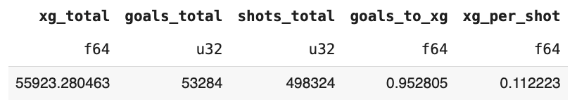
Those shots produced 53,284 goals from 55,923 xG, which works out to:

• Goals ÷ xG = 0.95

• xG per shot = 0.11

So yes—over the long term goals and xG do converge, albeit with a slight under-performance relative to the model.

---

2 — The High Scorers

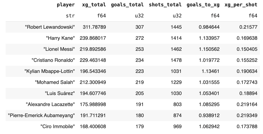
Across those 11 seasons, 39 players scored 100+ goals. Below are the top ten, ordered by total goals

Highlights:

• Lewandowski leads the raw count—307 goals from 312 xG (Goals ÷ xG = 0.98). Under the pundit logic of “must beat xG,” the Pole would be labelled an ‘under-performer’. Reality check: the metric and the man simply converge. And given his monstrous goals tally, the two percentage points are roughly in line with the model.

• Kane posts the first big outlier: 272 goals from 239 xG (+13 %), hinting at a repeatable team supply, striker movement, and finishing edge.

• Messi goes one better (253 ÷ 219 xG = 1.15).

• Ronaldo sits almost bang on expectation (1.02), while Mbappé mirrors Kane at 1.13 and Salah hovers just above par at 1.03.

So, in the top six we have:

• One “under-performer” (Lewandowski)

• Two basically on par (Ronaldo, Salah)

• Three genuine over-performers (Messi, Mbappé, Kane)

Not quite the narrative you get from weekend sound-bites, right?

---

3 — The Outliers

Among all 39 centurions, who really tops the Goals ÷ xG chart—and by how much?

Let’s sort the list by that Goals to xG ratio and see which names pop.

Surprised? Which headline grabs you more:

• Son Heung-min perched at No. 1 (elite was a given, but this screams world-class),

• Dries Mertens sliding into second, or

• Liverpool “flop” Iago Aspas ranking as more clinical than Messi?

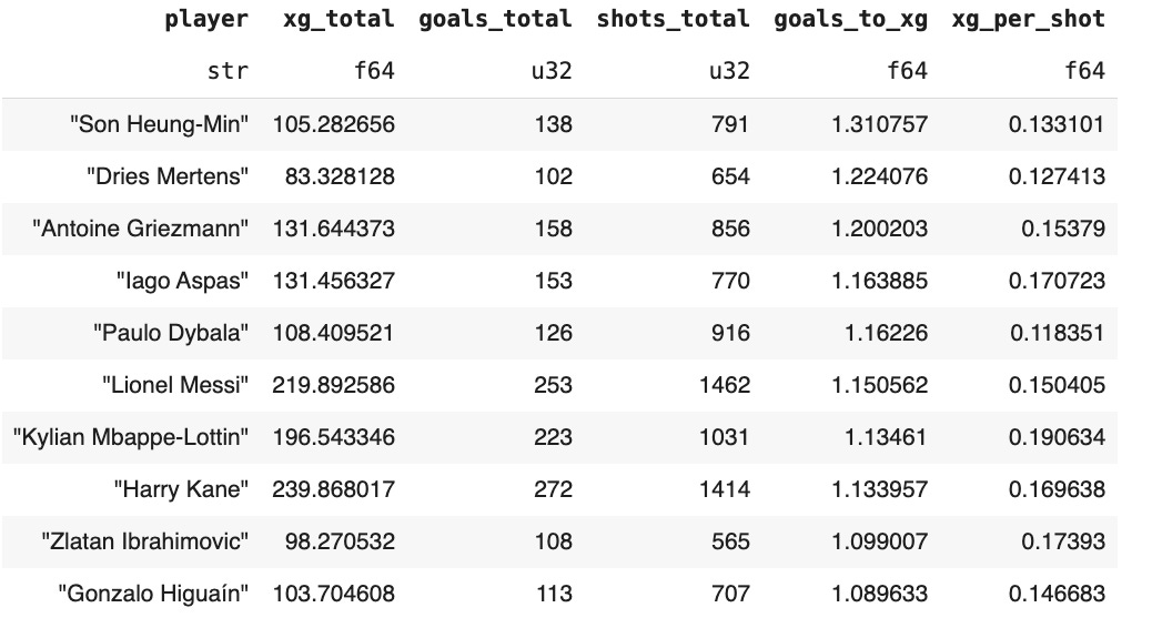
So we can say that 25 of 39 hundred-plus goal scorers posted a Goals ÷ xG ratio above 1.00.

• Son Heung-min leads the pack: 138 goals from 105.3 xG across 791 shots. That’s a 1.31 ratio—scoring 31 % more than an average player would from the same shots. That’s ridiculous. As in ridiculously good.

• Mertens (+22 %) and Griezmann (+20 %) round out the podium.

• Aspas and Dybala sit at +16 %, with Messi just behind on +15 %.

These are the rare finishers James Tippett had in mind: the tiny cohort who consistently bend the xG curve in their favour.

Notice how slim the margins are—outperforming by 9 % over a decade is enough to put you among the sport’s most efficient shooters (according to our initial definition, which of course is open to debate).

For everyone else, goals and xG converge exactly as the model expects.

Speaking of every else, what about the 14 players that scored 100+ goals but underperformed the xG?

---

4 — The ‘Underperformers’

So who sits at the other end of the scale—the lads who score plenty but should have scored more, given the chances they had?

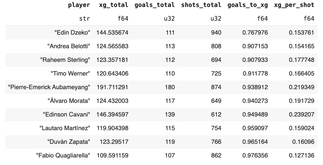
Among the 39 centurions, 14 finished below expectation. Here are the “bottom” ten:

Highlights:

• Edin Džeko is the starkest outlier: 111 goals from 145 xG (Goals ÷ xG = 0.77). That’s a 23 % shortfall (compared to what the average player would score from the same shots)—ouch.

• Lautaro Martínez (0.96) and Aubameyang (0.94) under-shoot, but only by single-digits—well within normal noise.

• Timo Werner’s 0.91 fits the eye test from his Premier-League spell: excellent movement and supply, finishing not quite matching the volume of chances?

---

5 — What does it all mean?

1. Goals and xG converge over multi-season samples—even for superstars. That’s exactly what a well-trained (xG) model should do actually.

2. Short-term spikes still matter. A player running hot (Goals ≫ xG) is probably in form, but the burst may owe as much to team supply and a bit of luck as to pure finishing.

3. For true clinical skill, use xGOT − xG.

   • xG = opportunity quality.

   • xGOT = execution quality.

   • Shooting Goals Added (xGOT − xG) strips out the noise and isolates finishing talent. We’ll tackle that metric in a future deep dive.

xG isn’t about “clinicalness.”

It blends team service, striker movement, and finishing edge into a single probability.

Next time you hear “he’s so clinical—look at his goals versus xG,” reach for xGOT instead.

And finally here’s how to reproduce this analysis in Python.

---

6 — The Python Corner

So, how do you reproduce this analysis?

First things first. If you’re new to Python, head to Google Colab—the quickest, zero-setup route (all you need is a Gmail account). Open a new notebook and you’re ready to roll.

You can download the code I’m about to detail here:

Install and import the packages

We’ll use soccerdata by Pieter Robberechts to pull Understat data and Polars for lightning-fast data wrangling.

!pip install soccerdata
import polars as pl
import soccerdata as sd

Define the study scope

Create lists for the leagues and the seasons you want to cover.

leagues = ['ENG-Premier League', 'ESP-La Liga', 'FRA-Ligue 1',
           'GER-Bundesliga', 'ITA-Serie A']

seasons = ['2014/2015', '2015/2016', '2016/2017', '2017/2018',
           '2018/2019', '2019/2020', '2020/2021', '2021/2022',
           '2022/2023', '2023/2024', '2024/2025']

Collect the shot-level data

sd.Understat and understat.read_shot_events() fetch every shot event for a given league-season pair. Eleven seasons across five leagues is roughly half a million shots, so expect the scrape to take up to an hour.

dfs_shots = []
for season in seasons:
    for league in leagues:
        understat = sd.Understat(leagues=league, seasons=season)

        df_shots = understat.read_shot_events()

        df_shots = pl.from_pandas(df_shots, include_index=True)

        df_shots = df_shots.with_columns([
            pl.lit(league).alias("league"),
            pl.lit(season).alias("season")])

        dfs_shots.append(df_shots)

Align columns and concatenate

Column sets can vary slightly from season to season, so we harmonise them before stitching everything together.

col_order_shots = []
for df in dfs_shots:
    for c in df.columns:
        if c not in col_order_shots:
            col_order_shots.append(c)

aligned_shots = []
for df in dfs_shots:
    missing = [c for c in col_order_shots if c not in df.columns]
    if missing:
        df = df.with_columns([pl.lit(None).alias(c) for c in missing])
    aligned_shots.append(df.select(col_order_shots))

shot_events = pl.concat(aligned_shots, how="vertical")

Big-picture aggregates

Total goals, total xG, shots, plus the global ratios:

(
    df_raw
    .with_columns(
        (pl.col("result") == "Goal").alias("goal"))
    .select(
        pl.col("xg").sum().alias("xg_total"),
        pl.col("goal").sum().alias("goals_total"),
        pl.col("shot_id").count().alias("shots_total"))
    .with_columns(
(pl.col("goals_total")/pl.col("xg_total")).alias("goals_to_xg"),        (pl.col("xg_total")/pl.col("shots_total")).alias("xg_per_shot"))

)

Player-level summary

Aggregate by player and compute Goals ÷ xG and xG per shot.

df_shots = (
    shot_events
    .with_columns(
        (pl.col("result") == "Goal").alias("goal"))
    .group_by(["player"])
    .agg(
        pl.col("xg").sum().alias("xg_total"),
        pl.col("goal").sum().alias("goals_total"),
        pl.col("shot_id").count().alias("shots_total"))
    .with_columns(
      (pl.col("goals_total")/pl.col("xg_total")).alias("goals_to_xg"),
      (pl.col("xg_total")/pl.col("shots_total")).alias("xg_per_shot"))
)

Slice the interesting bits

Top scorers (≥ 100 goals):

(
    df_shots
    .filter(pl.col("goals_total") > 100)
    .sort("goals_total", descending=True)
    .head(10)
)

Best Goal ÷ xG ratios among those centurions:

(
    df_shots
    .filter(pl.col("goals_total") > 100)
    .sort("goals_to_xg", descending=True)
    .head(10)
)

Worst Goal ÷ xG ratios among those centurions:

(
    df_shots
    .filter(pl.col("goals_total") > 100)
    .sort("goals_to_xg")
    .head(10)
)

Boom—that’s the myth of the “clinical” striker, reproduced in your own notebook.

If you found this issue useful, please share it!

You now know why even world-class forwards don’t always beat their xG, why that doesn’t make them wasteful, and what 11 seasons of data reveal about true finishing outliers.

Until next week,

Martin

The Python Football Review