How Soon Can You Trust the League Table?

And what 10 seasons of data reveal about when standings converge.

Hi friend,

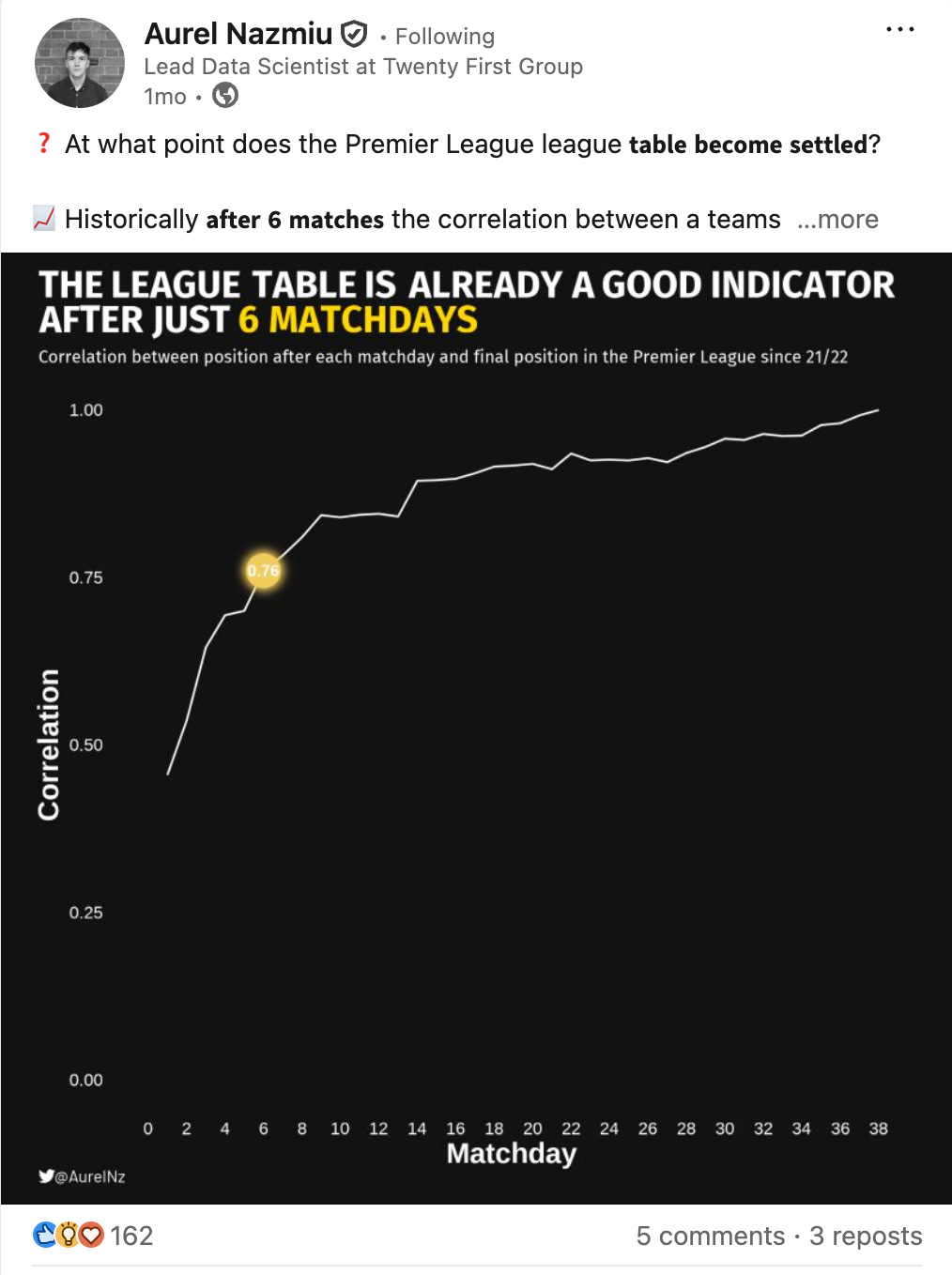
A few weeks back, Aurel Nazmiu shared a great visual showing when the Premier League table stabilises during the season.

Source: Linkedin

I loved it for three reasons:

1. It shows you don’t need fancy, complicated charts to do good analytics.

2. This seemingly simple graph hides a surprising (to a beginner) amount of data wrangling beneath the surface.

3. And when you try to recreate it yourself, you naturally start asking deeper questions you never considered when you first saw the figure — like what type of correlation should I use, and why does that matter? (more on that below).

Welcome to The Python Football Review #016.

In today’s edition, we’ll replicate that figure, then extend it to Europe’s top five leagues to see which ones settle earlier than others.

And along the way, you’ll see that a huge chunk of visualisation actually happens before you ever touch matplotlib — and why the classic (Pearson) correlation doesn’t work well with ranks (so we’ll use Spearman instead).

Let’s dive in.

---

So, what’s the plan, Martin?

We’ll start by collecting 10 seasons of Premier League results data. Then we’ll wrangle it into a dataset that contains each team’s league position at every matchweek, along with a variable for each team’s final-season position. Once we have that, we’ll calculate the Spearman correlation and finally plot the results.

Without further ado, let’s collect some data.

---

1 — Collecting the Data

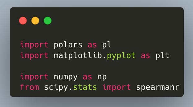
First, we import the libraries we’ll use. Polars for fast, readable wrangling. NumPy for small numeric utilities. Matplotlib for plotting. And SciPy’s spearmanr to compute the Spearman rank correlations between interim and final league positions.

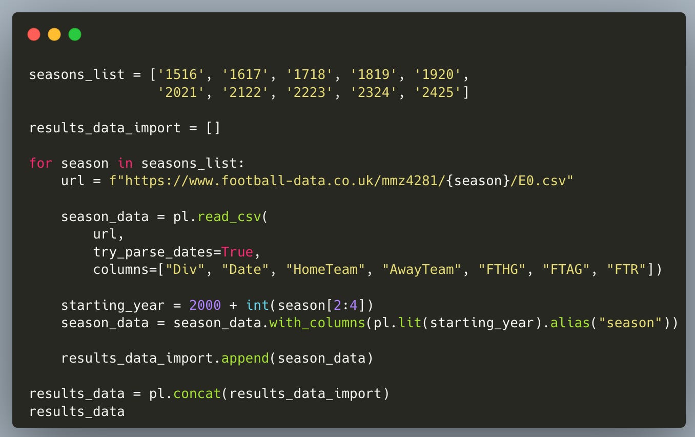
We’ll collect 10 seasons of Premier League results from Joseph Buchdahl’s Football-Data.co.uk — a fantastic open resource with historical match CSVs. With Polars’ read_csv, we can load them directly.

Here’s what the following snippet does:

• Defines the list of the 10 seasons we want.

• Creates an empty list to store each season’s table.

• Loops over each season and loads the corresponding CSV.

• Keeps only the relevant columns: date, home team, away team, full-time result, full-time goals.

• Adds a season column so we can track each row back to its year.

• Appends each cleaned table to our list.

• Concatenates everything into one big DataFrame.

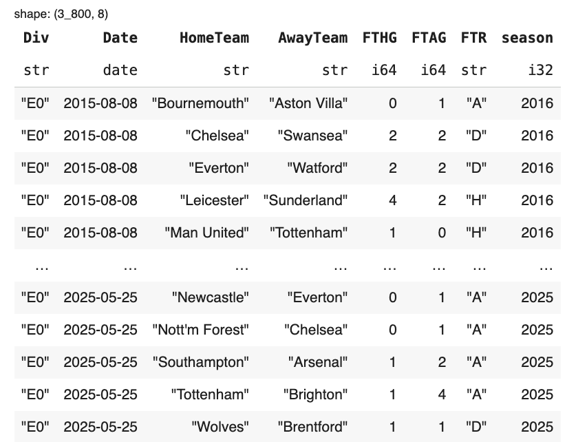
The result is a clean Polars table with one row per match, ready for wrangling.

2 — Wrangling

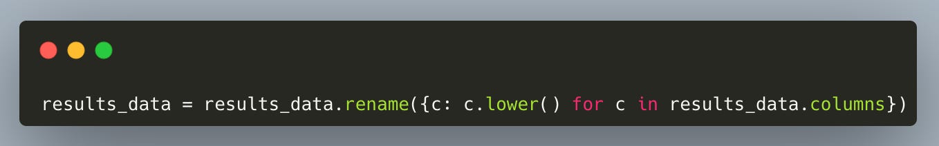
We start by renaming all columns to lowercase.

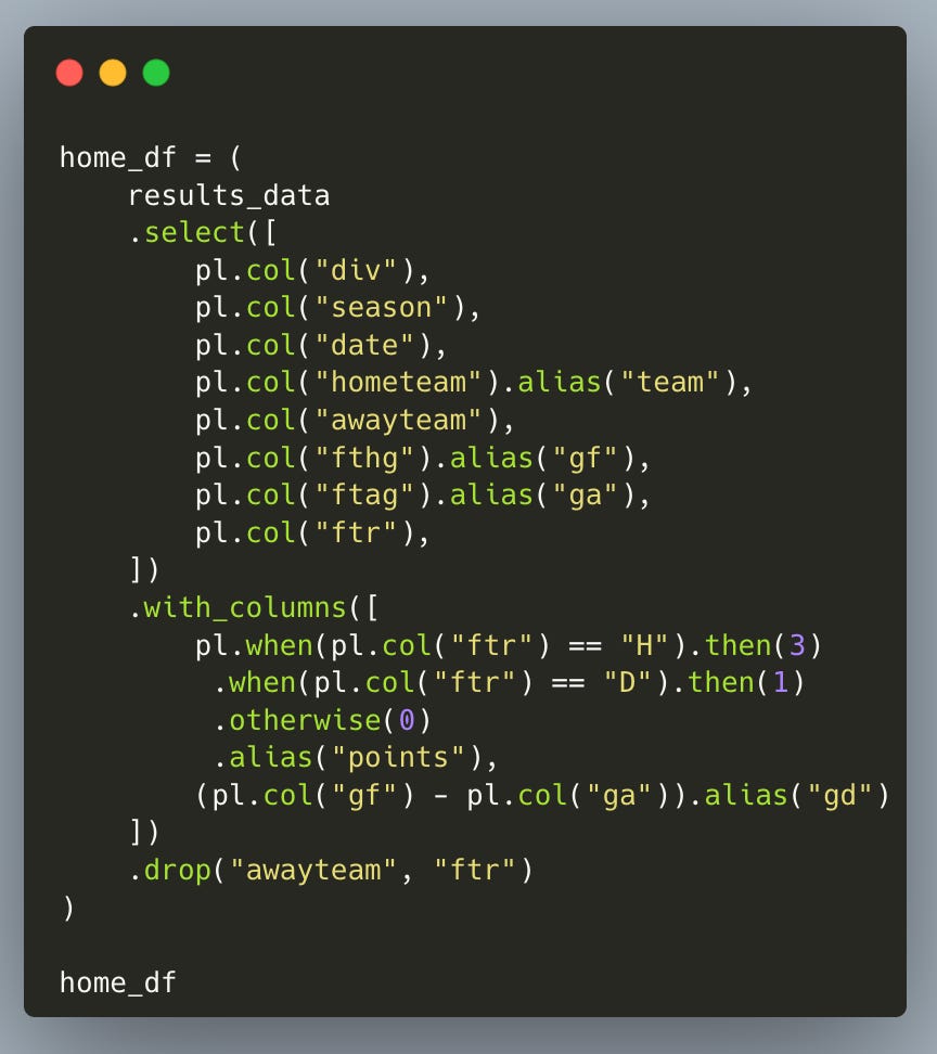
Next, we build the team-level data. For each home team, we calculate their goals for, goals against, points won, and goal difference.

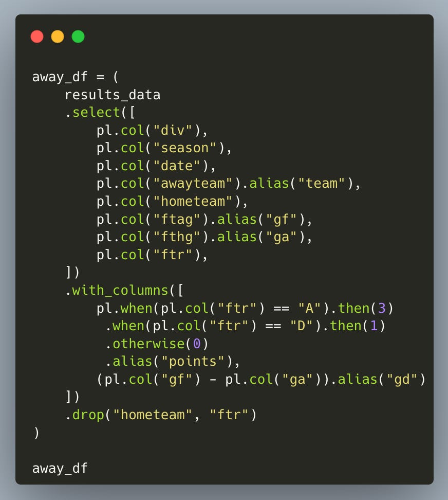
We repeat the same for each away team.

Then we stack the two together using a concatenation.

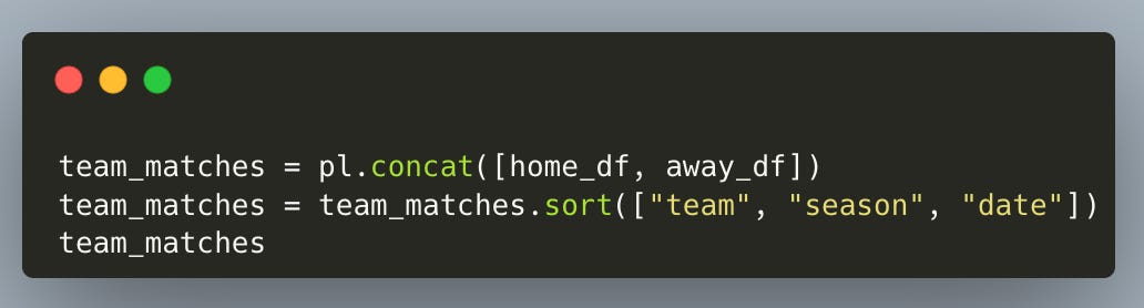
And now we have one row per team per match, containing that team’s goals for, goals against, points earned, and goal difference.

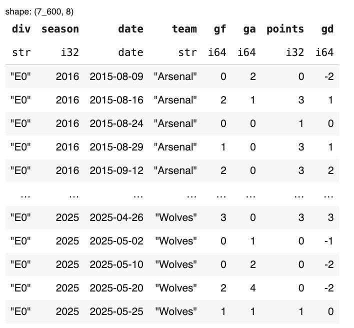
Since our data is ordered by date, we create a matchweek number. Yes — this is a simplification because not all teams play on the exact same day, but over 10 seasons this should not meaningfully impact the results.

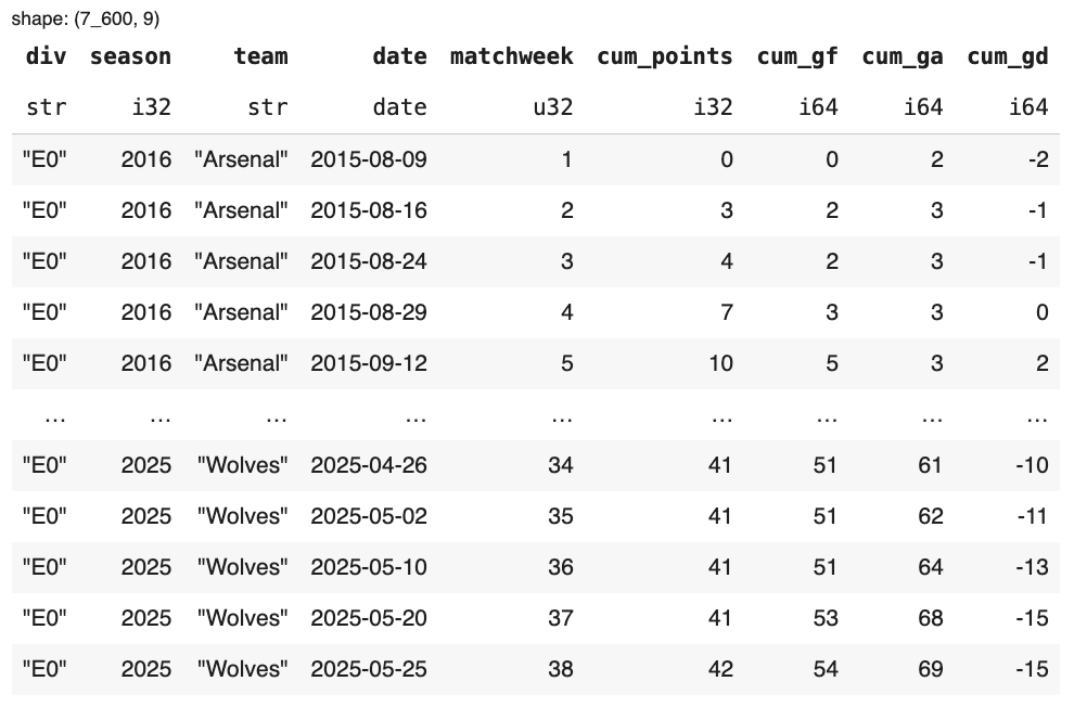
In addition to matchweek, we compute: cumulative points, cumulative goals for, cumulative goals against, cumulative goal difference.

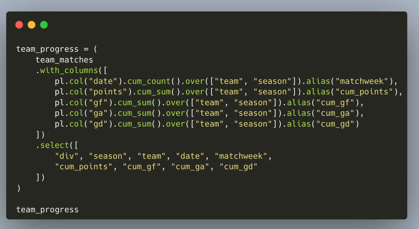
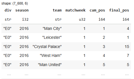
This produces a tidy table showing, for every team in every season, how their totals evolve after each matchweek.

Ranking the teams each week

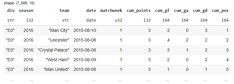
Based on the interim values for points accumulated, goals for, goals against, and goal difference, we create each team’s position for every matchweek. We do this by sorting first by points, then by goal difference, and finally by goals for.

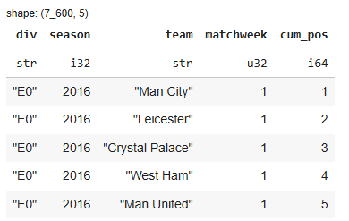
This new cum_pos column is what we care about.

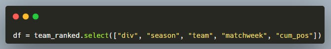
With our clean data ready, we move into the analytical phase. First, we select only the columns we need for the correlation exercise.

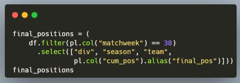
Then we create a final positions table by keeping only the last matchweek of each season — these are the official final ranks.

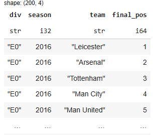
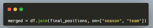
Finally, we join the final positions back to all matchweeks, so for any given matchweek, we can compare a team’s current position vs its final position.

Correlation over time

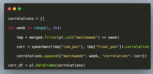
Next, we compute the correlation for each matchweek. The loop:

• takes matchweek k

• extracts all team positions at that point

• compares them to the final table

• computes Spearman’s ρ

Why Spearman and not Pearson (the classic correlation you first learn at school)?

• Pearson works on raw numeric distances — it assumes linear relationships, not ranks.

• Spearman works on ranks, which fits league tables perfectly. League positions are ordinal, not numerical — finishing 1st vs 2nd is not the same “distance” as finishing 10th vs 11th.

So Spearman is the right choice for football standings.

3 — Plotting

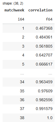
Once correlations are computed for all weeks, we plot them.

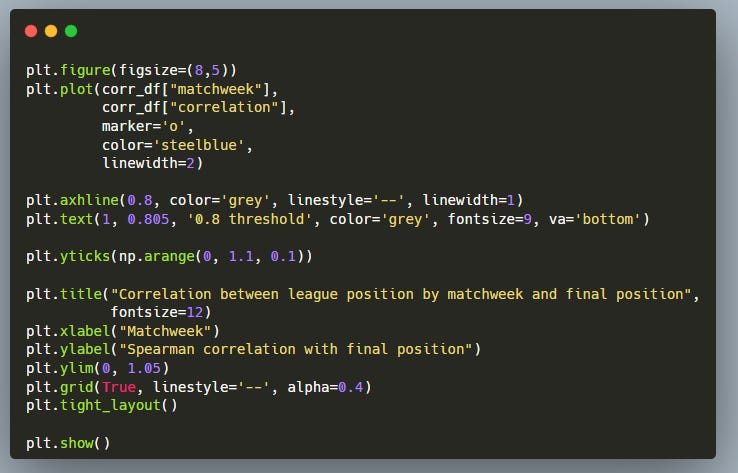
In competition economics (my day job), an 80% threshold is often used as a way to summarise a relatively strong effect or a reliable sample. I think it also links loosely to the Pareto idea — the 20% of factors that deliver 80% of the results. Regardless, for the purposes of this small article, we’ll treat 80% as the level where things start to “stabilise” (my newsletter, my rules).

So the natural question is:

At which matchweek does the Premier League’s correlation exceed 80%?

Answer: Around Matchweek 10.

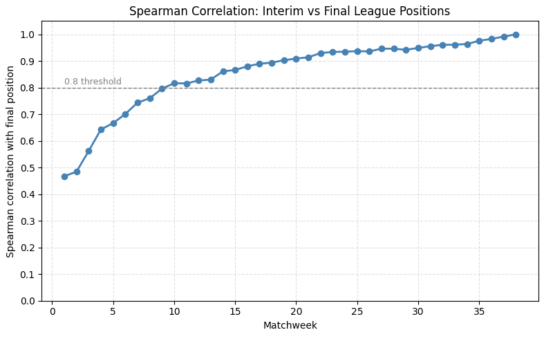
By that point, the table already starts to resemble its final shape to a meaningful degree. A few observations stand out:

• The 70% threshold is crossed as early as Matchweek 6.

• But it’s only around Matchweek 10 that the league passes the 80% mark — our “stability” line.

• And interestingly, crossing from 80% to 90% takes quite a bit longer. It’s only after roughly Matchweek 20 that the Premier League reaches the 90% correlation level.

• The final 10% — from 90% to 100% — takes about 18 additional matchweeks, almost half the season.

Early structure forms quickly. True stability takes time.

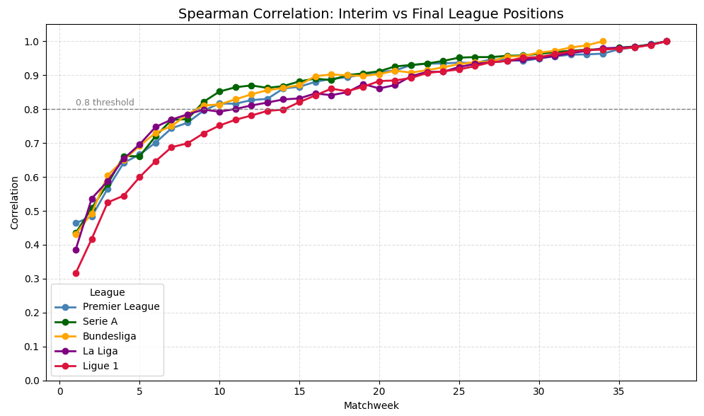
And what about the other Big 5 leagues?

It turns out:

• Ligue 1 crosses the 80% threshold only after Matchweek 15, and reaches the 90% mark around Matchweek 25 — a bit late.

• Serie A and the Bundesliga are the earliest to stabilise among the Big 5, passing the 0.8 threshold at Matchweek 9 — though La Liga and the Premier League aren’t far behind.

---

Boom — that was the behind-the-scenes look at when league standings actually settle.

You’ve now seen the amount of wrangling required to produce a graph that looks deceptively simple. You’ve seen the kinds of questions you end up asking only once you start working with the data (you’ve probably heard of correlation — but maybe not the difference between Pearson and Spearman). And you’ve learned that Ligue 1 takes its time to stabilise, while Serie A is the quickest of the Big 5.

This whole exercise reminded me of one of my favourite truths about (football) analytics: the best insights show up only once you’re deep in the weeds doing the work.

On paper, this looked like a trivial problem: “Compare matchweek positions to final positions. Plot the correlation.” Easy.

But once I started building the table — lining up matchweeks, ranking teams, joining final positions — a bigger question surfaced:

“Wait… what exactly is being correlated here? Do distances between positions even mean anything? No. So why am I reaching for Pearson? This is a ranking problem — of course Spearman is the right tool.”

You only see the true shape of a problem once you’re inside it.

Thanks for reading until the end.

See you next week,
Martin

---

As usual, you can grab the code below. The part that downloads all five leagues and plots the figure is included inside.

Simply download it, open a Google Colab session (if you don’t have Python installed), and run it line by line to replicate the analysis. And if you’re feeling adventurous, try switching the leagues and exploring beyond the Big 5.

Hint: you can use keys like E1 (Championship), E2 (League One), E3 (League Two), I2 (Serie B), SP2 (Segunda División), D2 (2. Bundesliga), F2 (Ligue 2), B1 (Belgium), P1 (Portugal), T1 (Turkey)… just to name a few.

Cheers!