
Expected Goals (xG) 101
What xG really measures (and what it doesn’t), the key misconception that trips up even seasoned pros, why its loudest critics are mostly wrong, and how to pull tons of xG data with Python.

Hi friend,
Welcome to The Python Football Review #001! 🎉
We’re kicking off with the stat that rewired football analysis—Expected Goals (xG). It’s quoted on broadcasts, splashed across Twitter infographics, and still sparks arguments every weekend.
By the end of this issue, you’ll know:
What xG really measures (and what it doesn’t)
The one misconception that trips up even seasoned pros
Why xG is a game‑changer—and why its loudest critics are (mostly) wrong. Looking at you, Jamie Redknapp.
How to pull xG data with a handful of Python lines (templates included)
Enjoy!
1 — So, What Is an Expected Goal?
Put simply, an expected goal (xG) is a value between 0 and 1 that measures how likely a shot is to become a goal. For example:
A long-range screamer might be
0.01 xG(1% chance).A tap-in could be
0.92 xG(92% chance).
Or more formally, xG quantifies the probability of a shot converting into a goal before the ball is struck.
That last piece is crucial: xG is fundamentally a pre-shot probability, not strictly a finishing metric. It’s a chance-creation measure, capturing how effectively a player (and by extension a team) reaches dangerous zones into one distilled value.
Case in point: Remember those two screamers Declan Rice scored in the first-leg quarter-final against Real Madrid?

The second one had an xG value of 0.06. That means if an average player attempted that same free-kick 100 times from 27 yards out, only 6 would typically go in. Yet Rice nailed it.
(And don’t get me started on the fact that he’d taken just 9 free kick shots in his entire professional career before attempting those two against the reigning European champions.)
That’s the power—and fun—of xG. It highlights when something is truly out of the ordinary.
But Martin, how do we actually decide it’s 6%, not 5% or 4%?
Glad you asked! xG providers (like Opta or StatsBomb) analyze hundreds of thousands of historical shots with similar conditions—distance to goal, angle, body part, defensive pressure, pass type leading to the occasion, position of the goalkeeper and more. Then they look at how often those shots were converted. And that’s basically it.
A few rules of thumb:
Closer to goal → higher xG
Wider shooting angle → lower xG
Headers generally have lower xG than footed shots
Penalties are worth about 0.79 xG
Different providers weigh these factors slightly differently, so you may notice small variations in xG values from one site to another (or as the famous saying goes … not all xG are created equal).
But, ultimately, xG shows how many goals an average team would be expected to score from those chances. It’s a measure of how good a shooting opportunity is, based on the historical likelihood that a similar shot ends in a goal.
2 — The Big Misconception: No More Than 1 xG per Attack
So far, you’ve learned that data providers assign an xG value to each shot. But how do we get a team’s (or a player’s) total xG for a match?
But Martin, don’t we just add up all the xG?
You’d think so, but that can overshoot reality. Here’s the issue.
A team can’t score more than one goal in a single attacking sequence. Let’s say we have a striker who attempted two shots in the same attacking sequence:
Shot #1:
0.45 xG(one-on-one with the keeper)Shot #2:
0.70 xG(rebound from the first shot on an open net)
If you just add them, you get 1.15, implying the possibility of more than one goal in that same possession—which is impossible.
To avoid inflated totals, data providers calculate the probability of no goal happening, then subtract that value from 1:
In our example, the chance of not scoring would be equal to = (1 - 0.45) × (1 - 0.70) = 0.55 × 0.30 = 0.165 meaning that there is a 16.5% chance of the attack not finishing with a goal.
And this leaves us with a 1 - 0.165 = 0.835 (83.5%) chance of the attack finishing with a goal.
Likewise, a single player can’t rack up 1.15 xG from one continuous attack. The provider caps the total at 0.835 (83.5%) for that sequence.
So, individual shots can still have 0.45 and 0.70 xG, but match stats will show the possession’s combined xG as 0.835.
Phew! I hope I did not lose you.
Long story short:
One shot? Use its xG “as is.”
Team or player totals? Data providers adjust to ensure no single attacking possession exceeds 1 xG.
Plenty of fans—and even some professionals—overlook this nuance. But now you know better!
3 — xG’s blind spot
Before I gush about the two ways xG changed football analytics, a quick reality check: xG isn’t perfect. It’s an aggregate measure—it doesn’t care who pulls the trigger or how the shot is struck.
xG rates the chance, not the shooter—a subtlety many people miss.
If the average conversion rate from a position is 30 %, that doesn’t mean every player finishes 30 % of the time. Gabriel Jesus might tuck them away 20 % of the time, while Erling Haaland buries 50 %.
And that’s the point: xG measures the quality of the chance, not the quality of the player on the end of it.
Still, fans and analysts love using the gap between Goals and xG as a finishing barometer. It’s handy—just easy to misread.
Remember, xG is assigned before contact. It shows how often a player gets into prime areas plus the historical finishing rate from those locations.
We’ll cover a sharper finishing metric—Expected Goals on Target (xGOT)—in a future issue. xGOT grades the strike after it leaves the boot. Until then, Goals − xG is fine—just know it blends chance quality and historical finishing.
4 — Two Reasons xG Revolutionized How We Think About Football
(a) xG Tells a Fuller Story Than Goals Alone
Goals are rare and don’t always reflect who actually controlled a match. A team might play poorly yet score a couple of lucky goals and win 2–0, while another team might dominate every aspect but fail to find the net.
xG reveals how many dangerous chances a team generated (and allowed). For instance:
A 2–0 win with an xG scoreline of 2.5–0.7 suggests the winning side not only finished well but also likely stifled the opponent.
A 2–0 win with an xG scoreline of 0.7–2.5 implies the hosts scored on minimal opportunities while the visitors simply couldn’t convert. Could be luck, poor finishing, or a brilliant goalkeeper.
And because xG captures this deeper performance nuance, it’s arguably (dare I say it) the most accurate predictor of future team (and player) success we currently have (according to the data providers, not just me).
But wait, Martin—doesn’t game state matter?
What if a strong attacking team scores two early goals, then sits back to protect its lead in the last 15 minutes? That scenario could let the opponents rack up a bunch of late xG, even though the attacking team stayed in control.
Exactly. That’s why nobody should rely on xG (or any other metric for that matter) in isolation. Context matters, so it’s best paired with xG match evolution graphs (which we’ll create in future newsletters) or deeper contextual analysis.
And finally, let’s not forget that defensive teams can still rack up xG: Even if you “park the bus,” you might create high-value counterattacks against fewer defenders—sometimes resulting in a surprisingly high xG.
(b) xG Separates Skill from Luck
The most common (early) critique of xG was: “If the real scoreline doesn’t match the xG, then xG is pointless!” But it’s actually the other way around: if the final score departs drastically from xG, that might indicate randomness or exceptional finishing/defending.
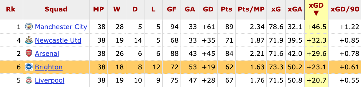
And that’s precisely why clubs like Brighton stuck with Graham Potter even during their disastrous (results-wise) 2020/21 season. The xG numbers showed they were creating—and conceding—chances at a level worthy of European qualification (as opposed to their actual 16th-place finish, just two spots above the relegation zone).

Over the long term, xG and actual goals tend to converge. Short-term luck—good or bad—can skew results for a while, but eventually, high-chance-creating teams rise, while those living on half-chances often slide.
And that’s exactly what happened with Brighton: by the 2022/23 season, the Seagulls finished 6th and earned a place in European football.
Over time, xG and actual goals tend to converge. A freak week, month, or even half‑season can bend the curve, but keep creating high‑value chances (and limiting the opposition) and the scoreboard will eventually fall in line.
In the long run:
Clubs that consistently outperform xG—Manchester City, peak Liverpool—aren’t “lucky”; they own a repeatable edge the model can’t quite capture.
Teams that habitually underperform xG are usually paying for poor finishing, shaky defending, tactical flaws, or endless managerial roulette.
Captain Obvious, at your service.
In the short run, though, you can dominate xG and still lose—and those are the matches pundits seize on to declare the stat “pointless.” Context is everything; one game is noise, a season is signal.
So, no, xG isn’t perfect, but it brings priceless nuance to any discussion of skill and luck. The problem isn’t that pundits misunderstand the metric; they misapply it.
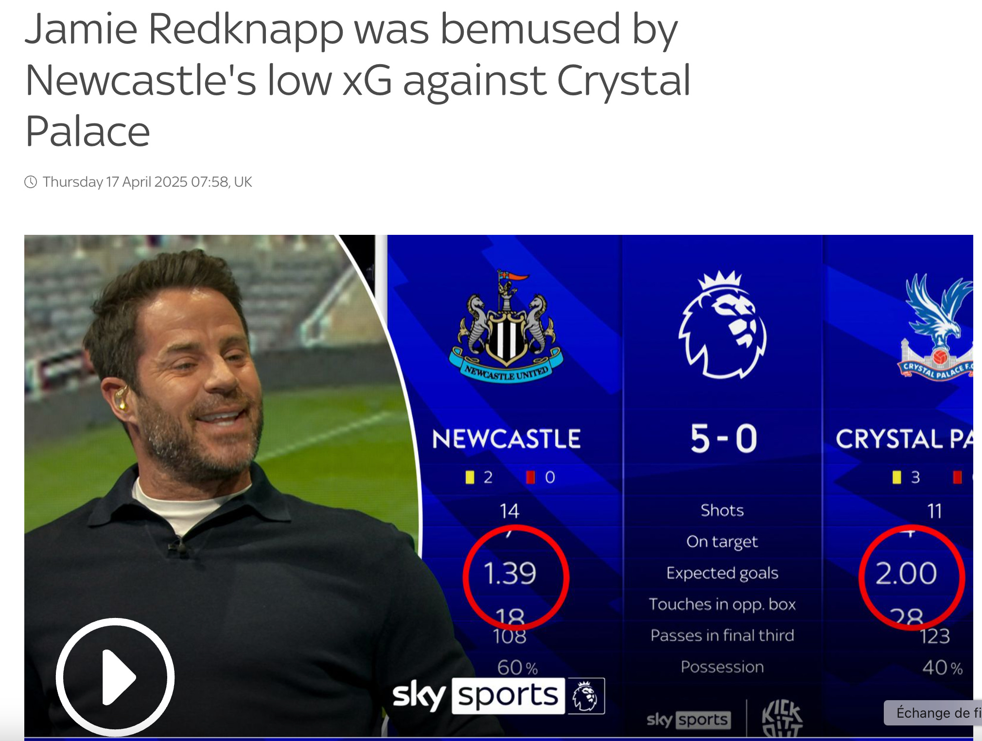
Cue Jamie Redknapp. After Newcastle thumped Crystal Palace 5–0, he scoffed at the Magpies’ modest 1.39–2.0 xG and declared, “xG is nonsense.”
Why the score and xG diverged
A big gap usually comes from one—or a mix—of three factors:
Clinical over‑performance — Freakish finishing, goalkeeper howlers, or own goals (which carry zero xG).
Cold under‑performance — Fluffed sitters, heroic saves, or a missed penalty (~0.79 xG down the drain).
Both of the above — One team red‑hot, the other ice‑cold.
Against Palace, Newcastle hit the perfect storm:
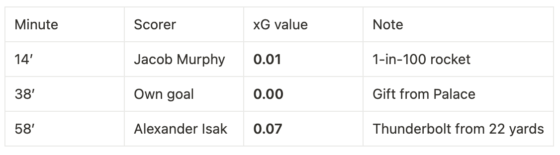
That’s three goals from just 0.08 xG.
Meanwhile Palace’s best moment—a penalty worth ~0.79 xG—clattered wide, and Newcastle’s defence swatted away two other high‑value shots.
So, Jamie, this wasn’t a straightforward 5‑0 masterclass; it was a cocktail of wonder‑strikes, an own goal, stout defending, and a blown spot‑kick. xG lays the pattern bare, even if you missed the live broadcast. 😊
Enough theory—let’s grab some data. Here’s how to download current and historical xG numbers with just a few lines of Python.
5 — How to Fetch xG Data Using Python
In this final section, you’ll learn how to download historical xG data from Understat.com using just a few lines of Python code.
If you’re completely new to Python, the easiest way to get started is with Google Colab—a free, cloud-based service that lets you write and run Python code directly in your browser, no setup required.
Go to https://colab.research.google.com and sign in with your Google account.
In the Colab dashboard, click File in the top menu, then select New notebook.
From there, you can type in the code I’m about to share, or simply download it from the link below.
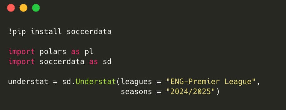
Now, let’s see how to get your hands on xG data. We’ll use a Python library called soccerdata (created by Pieter Robberechts), which makes collecting valuable stats quick and easy. You can learn more about it here.
First, install the soccerdata package. Then import it alongside our data-wrangling library of choice, polars❤️. Once that’s done, set your parameters. In the example below, we’re pulling xG data from the English Premier League for the current (as of writing) 2024/25 season.
Collecting Match-Level xG Data
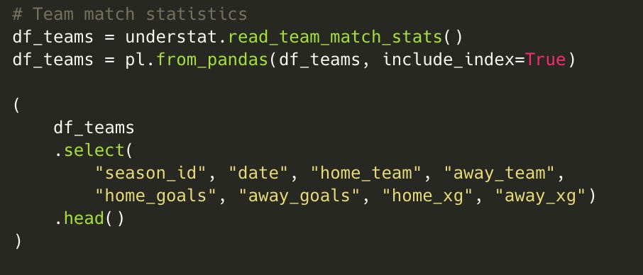
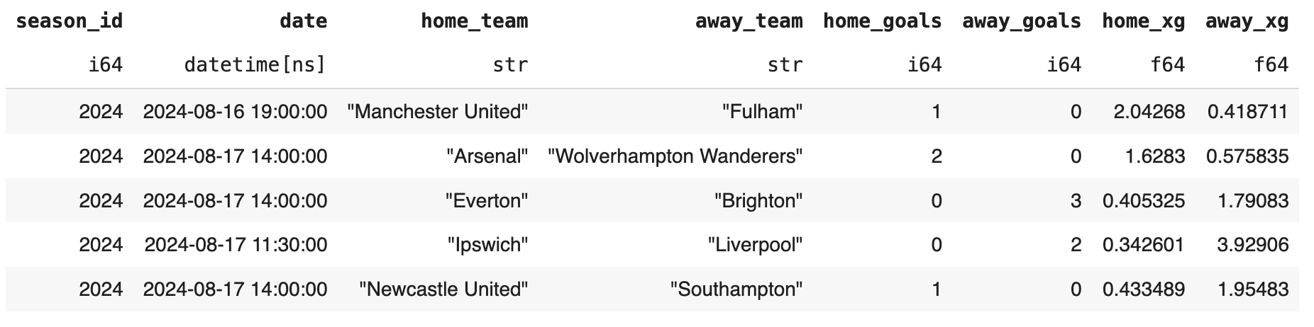
Next, let’s move on to the actual data collection. Here’s how you can pull match-level xG information. In the snippet below, we grab data for every game in the current season, focusing on the home and away teams’ goals as well as their respective xG figures. We also convert the resulting Pandas DataFrame into a Polars DataFrame to take advantage of Polars’ exceptionally easy, plain‑English expressions. (Stay tuned for a dedicated newsletter on this topic soon.)
Collecting Player-Level Match xG
The code snippet below fetches data for each player’s xG performance on a match-by-match basis. Here, we’ve filtered the results to show Bukayo Saka. You can see that in his first match of the season against Wolves, he scored 1 goal from 5 shots, with a total xG of 0.52.


Collecting Player-Level Season xG
The following snippet retrieves each player’s cumulative xG over the entire season. In this example, we observe that, at the time of writing, Bukayo Saka has accumulated 6.18 xG across 19 matches, scoring 6 goals in total.


Collecting Player-Level Shots xG
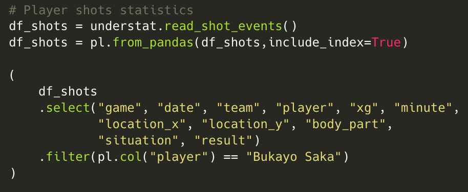
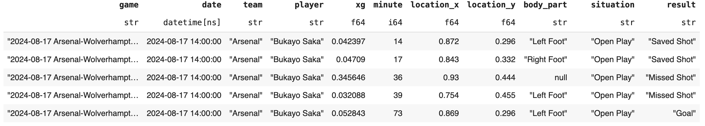
Finally, here’s how to access shot-level data for a specific player. In the snippet below, each of Bukayo Saka’s attempts is listed with details like shot location, xG value, body part used, the situation (e.g., open play or set piece), and the outcome (goal, saved, or missed).
It goes without saying that we’re only scratching the surface of what the soccerdata package can do—you can pull tons of other advanced metrics from it. But since this newsletter is already running long, I’ll let you explore the rest on your own.
Also note that you can access data going back to the 2014/15 season for all of Europe’s top five leagues by using these keys:
'ENG-Premier League''ESP-La Liga''FRA-Ligue 1''GER-Bundesliga''ITA-Serie A'
Boom! And that’s it for this first edition.
If you found this newsletter helpful, please spread the word! You now know how xG is calculated, what it measures, why it matters, how to avoid the “1.15 xG in one possession” pitfall, and how to grab valuable xG data in seconds.
I’m still experimenting with the format of the newsletter, so your feedback is super welcome—would you prefer shorter content, longer deep dives, more Python, or more football concepts? Or does this format hit the mark?
My aim is to build a truly practical newsletter together with you.
Until next week,
Martin
The Python Football Review
P.S. If you enjoyed this newsletter and want to support it, please consider sharing it on Twitter or LinkedIn. I know it can feel like a chore (I usually hesitate too), so to say thanks, I’ll send you an exclusive extended Python notebook that downloads 10 seasons of xG data from Europe’s top five leagues—fully automated and wrangled into one dataset ready for analysis. Just send me an email at martin@pythonfootball.com once you’ve shared, and I’ll send it over. Cheers!
Thanks for this and really enjoying the posts.
Do you have any advice on creating a model to measure xG with your own approximate coordinates for youth games or matches at lower levels.
I have used ChatGPT to develop something and it seems to hold up fairly well to existing models but would love to get your feedback.
Thank you again.
I am a beginner and the deep dive into the football concept along with real life examples really helps. It never felt like a long post. I was glued till the end. The python code snippets also helps because it provides a starting point for further analysis. Thank you for writing this post!