
Elliot Anderson and the Art of Showing Just Enough Data

So Josh Williams just tweeted this — a great little bit of football analytics on Sky Sports.

And it’s not the first time I’ve stumbled across Elliot Anderson’s name this season either.
So, since I’m officially back (after a long summer break), I thought — why not do a quick, improvised Python Football Review?
Welcome to The Python Football Review #013, where we’ll recreate Sky Sports’ figure in just a few minutes using Python.
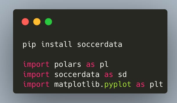
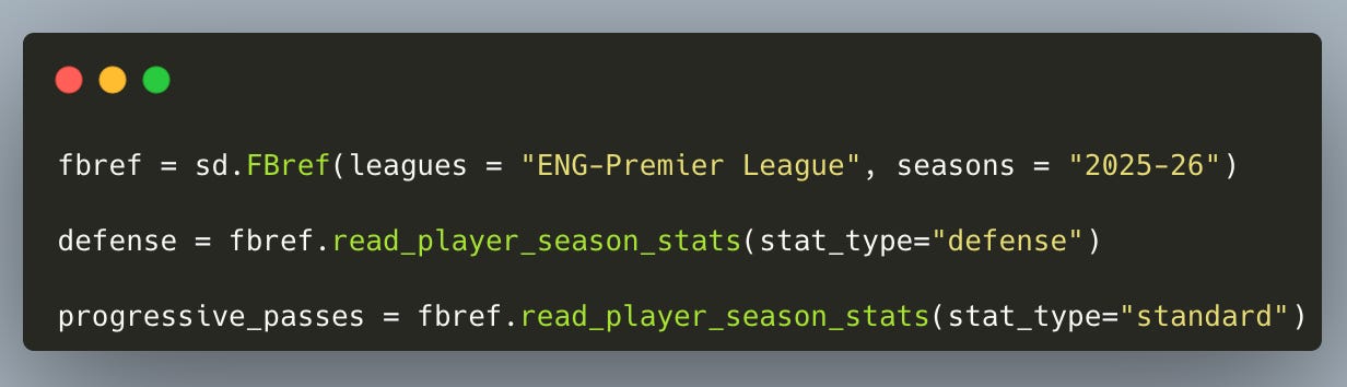
Step 1 — Collecting the Data
We’ll start with the basics. Install soccerdata to scrape data from Opta via FBref, and import it alongside polars (for easy wrangling) and matplotlib (for plotting).
From FBref, tackles live in the defensive stats, while progressive passes come from the standard stats. No, FBref doesn’t have line-breaking passes, but progressive passes are the closest we can get — so we’ll take them and move on.
Step 2 — Wrangling the Data
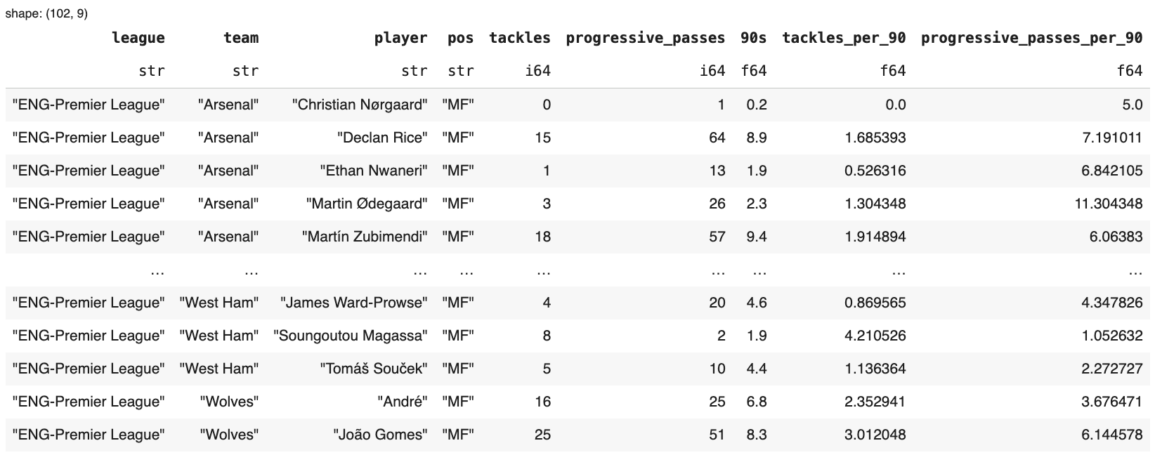
soccerdata returns pandas DataFrames, but I prefer working in Polars for its clarity. So, we convert everything to Polars, rename our columns of interest, and keep only what we need.
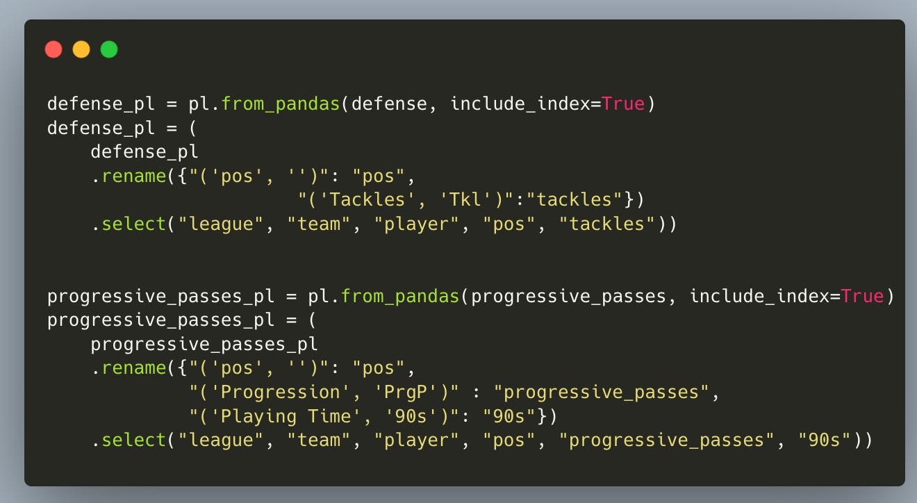
Next, we join the two datasets, create tackles per 90 and progressive passes per 90, and filter for midfielders only.
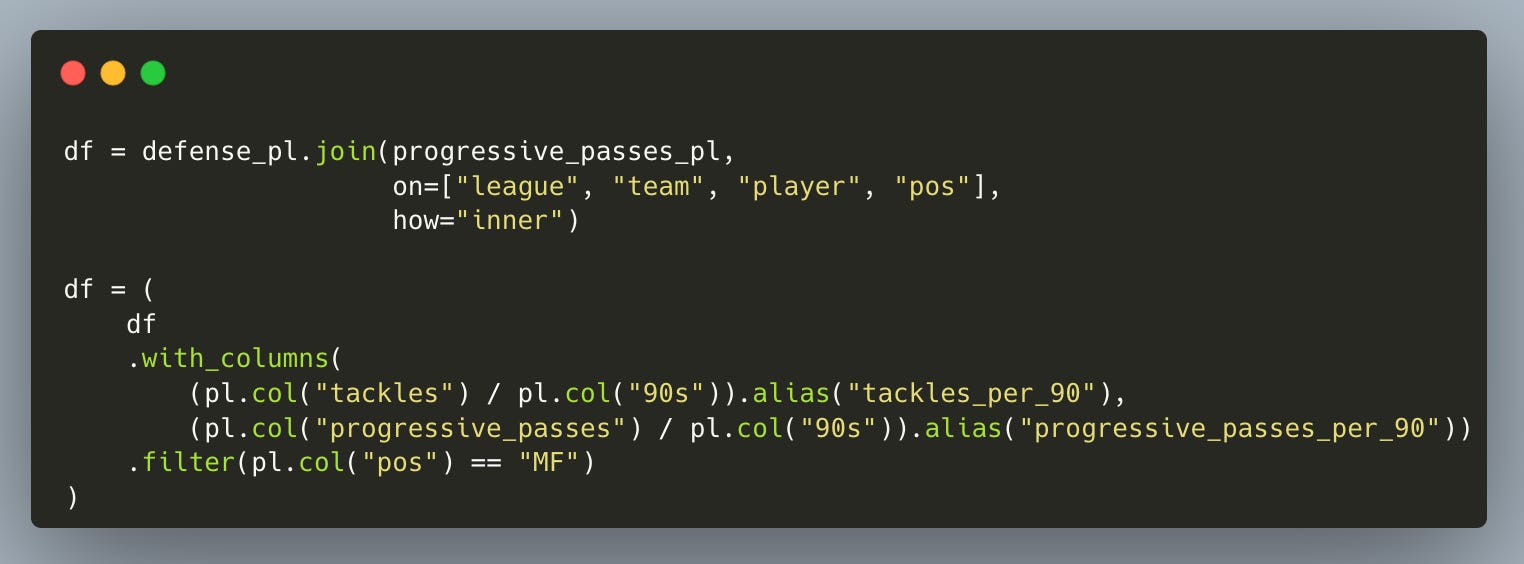
After this step, we’re left with a clean DataFrame of 102 midfielders — ready to visualize.
Step 3 — Visualizing
Now that we’ve got our cleaned dataset, it’s time for making the visual.
We’ll create a simple scatter plot, where each dot represents a player — progressive passes on the x-axis, tackles on the y-axis.
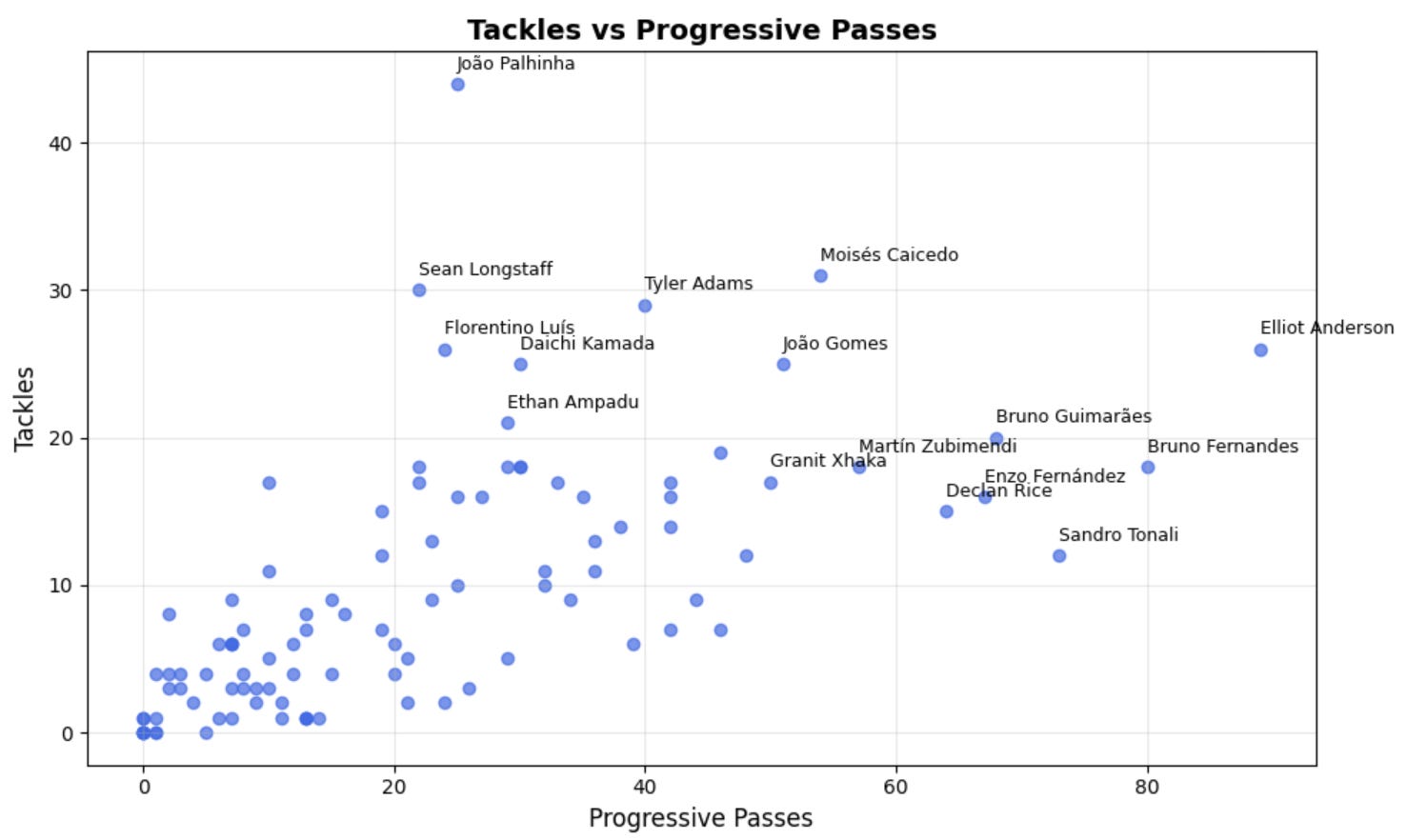
And here is our scatter plot.
Right away, Nottingham Forest’s Elliot Anderson jumps off the chart — an aggressive ball-winner (26 tackles) and an exceptional progressive passer (89 progressive passes).
If you look closely at Sky Sports’ version, you’ll see their metrics are per 90 minutes.
So, let’s replicate that too.
Once we adjust for minutes played, Anderson still stands out — averaging 8.9 progressive passes and 2.6 tackles per 90 minutes. But he’s no longer quite the outlier he appeared to be in the first figure.
What happened? Well, some players in the dataset likely have played far fewer games than he has — which naturally inflates their per-game averages.
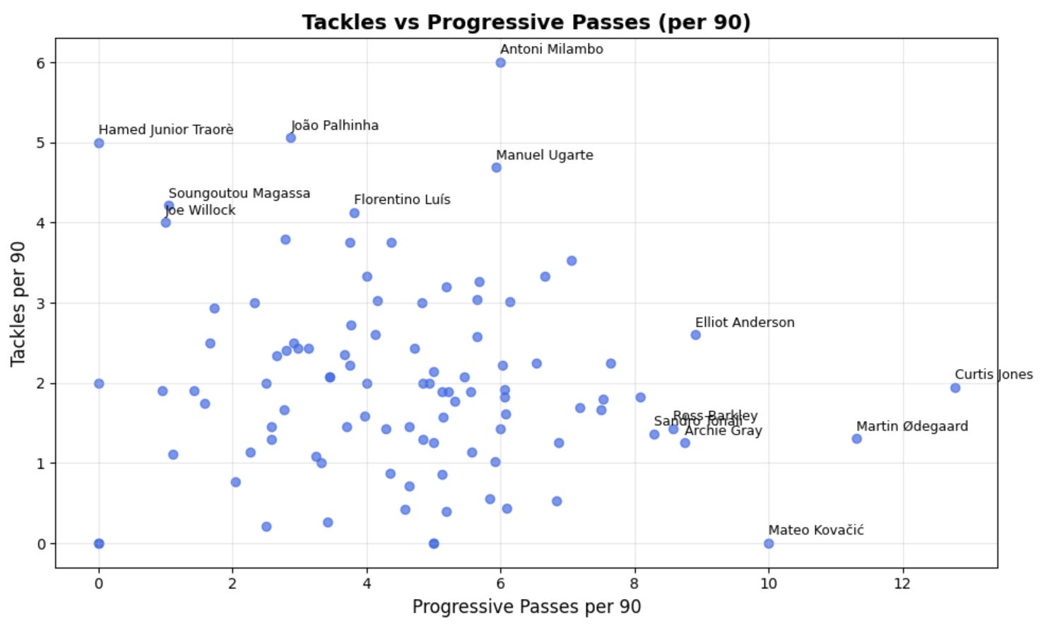
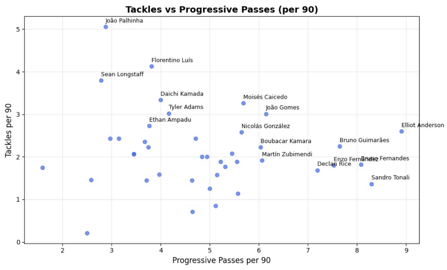
So, once we account for that (for example, by keeping only players who’ve played at least six matches), we end up right where we expected to be from the start.
This small exercise is a great reminder of what matters when visualizing data.
It’s not just about plotting numbers — it’s about making sure the sample is representative. Because if you include everyone without context, outliers can easily distort the message.
It’s also a reminder that with the right filters, you can subtly shape which stories (and which players) stand out (I am not saying that’s the case here). That’s why even Sky’s version says “selected midfielders.” Filtering matters. (And kudos to them for making that clear).
Anderson is an exceptional player. Sky Sports are a trusted source. This little project simply serves as a reminder of the dos and don’ts in data visualization. Here, everything is perfectly valid — but it also shows how, depending on the filters you use, the picture can shift.
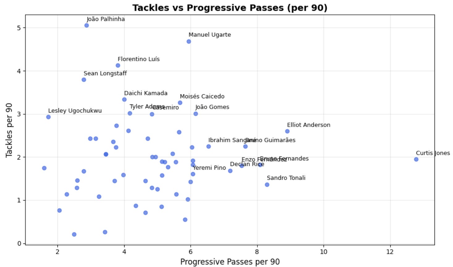
Here’s the same figure again, this time keeping only players who’ve played at least three full matches — which is still a fair cut-off (roughly 30% of the season so far).
So Curtis Jones for Player of the Season? Maybe not (yet?) … but you get the point.
Wrapping Up
This was a small but fun reminder of two things:
With Python, you can recreate Sky Sports-worthy analytics visuals in minutes (even if the Matplotlib aesthetics we used here still lag a bit behind).
Data always needs context — even the cleanest chart can mislead if you forget to filter carefully. (Not that I’m saying there’s one “proper” filter here — but you see what I mean)
And with that, we wrap up this short, improvised edition of the Python Football Review.
Ah — it feels so good to be back.
Thanks for reading,
Martin
P.S. As usual, you can grab the code below.
Great post, Martin.
Question I'm getting the FBref Response Code 403 in the collecting data step. Did they change their web scrapping policy recently?